
Much of the fun of an amusement park ride results from its stomach-churning, mind-jangling unpredictability. The Tilt-A-Whirl, for example, spins its passengers in one direction, then another, sometimes hesitating between forays and sometimes swinging abruptly from one motion to another. A rider never knows exactly what to expect next.
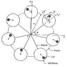
Yet these complicated, surprising movements arise from a remarkably simple geometry. A passenger rides in one of seven cars, each mounted near the edge of its own circular platform but free to pivot about the center. The platforms, in turn, move at a constant speed along an undulating circular track that consists of three identical hills separated by valleys, which tilt the platforms.
The platform movements are perfectly regular, but the cars whirl around independently in an irregular manner. Moreover, there is essentially just one adjustable parameter–the rate at which the platforms move around the track.
When the platforms travel at very low speeds, the cars complete one backward revolution as their platforms go over each hill. In contrast, at high speeds a car gets slammed to its platform’s outer edge and stays locked in that position. In both cases, the motion is predictable.
What happens at intermediate speeds?
To model dynamical systems like the Tilt-A-Whirl, mathematicians, scientists, and engineers use equations that describe how the positions and velocities of a system and its components change over time in response to certain forces.
It’s convenient to characterize a system’s dynamics by plotting how its position and velocity evolve over time. Each plotted point represents the system’s state of motion at a particular instant, and successive points generate a winding line through an imaginary mathematical space (known as phase space) representing all possible motions. Different starting points generally initiate different curves.
A simple, repeating motion, like the to-and-fro oscillations of a swinging pendulum, appears as a circle or some other closed curve. Such a plot shows that the system cycles through precisely the same state of motion again and again at regular intervals.
More complicated sequences of movements produce tangled paths that wander through phase space, sometimes never forming a closed loop.
Often, it helps to examine such complicated movements not at every moment but at predetermined, regular intervals. In other words, you start with a point representing the system’s initial state, then wait a given time and plot a second point to give the system’s new state, and so on.
In the case of a simple pendulum, selecting an interval equal to the time it takes the pendulum to complete one oscillation produces a plot that consists of a single point. The pendulum is always back in its initial state at every repeated glimpse of its motion.
When the motion is chaotic, however, there is no characteristic period. The resulting plot, known as a Poincaré section, shows points scattered across the plane–like bullets puncturing a sheet of paper. In a sense, the system is continually shifting from one unstable periodic motion to another, giving the appearance of great irregularity.
To describe the Tilt-A-Whirl’s dynamics, physicists Bret M. Huggard of Northern Arizona University and Richard L. Kautz of the National Institute of Standards and Technology found a mathematical equation that approximates the motion of an idealized Tilt-A-Whirl. In essence, the movements of an individual car resemble those of a friction-impaired pendulum hanging from a support that is both rotating and being rocked back and forth while the pendulum swings. Solving the equation determines how a Tilt-A-Whirl car would behave under various conditions.
To find out what happens at intermediate Tilt-A-Whirl speeds, Kautz and Huggard plotted a set of points representing the velocity and angle of a car at the beginning of each of 100,000 tilt cycles. They found that the values never repeated themselves but were scattered in a distinctive swirling pattern confined to a portion of the plane.
For these platform velocities, even slight changes in starting point lead to radically different sequences of points. At the same time, it becomes virtually impossible to predict several steps ahead of time precisely what will happen. Such sensitive dependence on initial conditions stands as a hallmark property of chaos.
Hence, what happens to an individual Tilt-A-Whirl car is highly dependent upon the weight of its passengers and where they sit. The resulting jumbled mixture of car rotations never repeats itself exactly, which gives the Tilt-A-Whirl its lively and unpredictable character. Indeed, no two trips are ever likely to produce exactly the same thrills and chills.
Interestingly, the mathematical model used by Kautz and Huggard predicts that chaotic motion would occur at a speed close to the 6.5 revolutions per minute at which the ride is normally operated.
“A walk around an amusement park suggests that several other common rides display chaotic behavior similar to that of the Tilt-A-Whirl,” Huggard and Kautz note. Typically, rides that fit this category have cars that are free to rotate or shift back and forth as they follow a fixed track.
The Tilt-A-Whirl first operated in 1926 at an amusement park in White Bear Lake, Minnesota. Most likely, the ride’s inventor, Herbert W. Sellner, discovered its unpredictable dynamics not through mathematical analysis but by building one, trying it out, and making trial-and-error adjustments.
“Ride designers have been fairly adept at finding chaos without appreciating the mathematics underpinning what they’re doing,” Kautz notes. The situation is changing, however. To fine-tune the thrills, manufacturers are beginning to take advantage of mathematical analyses and computer simulations to help build chaotic motion deliberately into amusement park rides.


